

How to Use IF Statements in Spreadsheets (Plain-English Guide)
- Peter J.

- Jul 3
- 5 min read
The IF function checks whether a condition is true or false, then shows a different result depending on the answer. The syntax is: =IF(condition, value_if_true, value_if_false). For example, =IF(B2>50, "Pass", "Fail") shows “Pass” if the value in B2 is greater than 50, and “Fail” if it’s not.
This is one of the most powerful and frequently used functions in any spreadsheet. Once you understand IF, a whole new level of spreadsheet capability opens up.
Understanding IF in Plain English
Think of IF as a yes/no question:
“IF this is true, show me this. Otherwise, show me that.”
Real examples:
IF sales are above $10,000, show “Bonus.” Otherwise show “No Bonus.”
IF a task is marked Done, show “Complete.” Otherwise show “Pending.”
IF a score is 60 or higher, show “Pass.” Otherwise show “Fail.”
Each one follows the exact same structure.
The Syntax
=IF(condition, value_if_true, value_if_false)Part | What it means |
condition | The test you want to run. Usually a comparison: A1>10, B2="Yes", C3<>"" |
value_if_true | What to show when the condition is true. Can be text (in quotes), a number, or another formula. |
value_if_false | What to show when the condition is false. Same options. |
Your First IF Formula
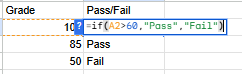
Say you have a column of test scores in column B, and you want column C to say “Pass” or “Fail” based on whether the score is 60 or above.
Click cell C2 and type:
=IF(B2>=60, "Pass", "Fail")Breaking it down:
B2>=60; the condition: is B2 greater than or equal to 60?
"Pass"; show this text if yes
"Fail"; show this text if no
Press Enter. The cell shows “Pass” or “Fail” based on the score in B2.
Now copy C2 down the column to apply the formula to all your rows. Because B2 is a relative reference, it adjusts to B3, B4, B5, and so on.
Comparison Operators You Can Use
Operator | Meaning | Example |
> | Greater than | B2>100 |
< | Less than | B2<0 |
>= | Greater than or equal to | B2>=60 |
<= | Less than or equal to | B2<=50 |
= | Equal to | B2="Done" |
<> | Not equal to | B2<>"Done" |
Note: When comparing text, put it in double quotes. When comparing numbers, don’t use quotes. =IF(A1=5, ...) works, but =IF(A1="5", ...) checks if A1 contains the text character “5,” not the number 5.
Using IF with Numbers as Results
Your IF formula doesn’t have to return text. It can return numbers, do calculations, or reference other cells.
=IF(B2>100, B2*0.1, 0)This gives a 10% bonus if sales (in B2) exceed 100, and gives 0 otherwise.
=IF(C2="Done", "", D2-TODAY())This shows nothing (empty text "") if a task is done, or calculates days remaining if it’s not.
Nested IF: Checking More Than Two Outcomes
What if you have more than two possible results? You can put one IF inside another. This is called a nested IF.
Example: Grade letter based on score.
90+ = “A”
80-89 = “B”
70-79 = “C”
Below 70 = “F”
=IF(B2>=90, "A", IF(B2>=80, "B", IF(B2>=70, "C", "F")))Breaking it down:
First, check if B2 is 90 or above → “A”
If not, check if it’s 80 or above → “B”
If not, check if it’s 70 or above → “C”
If none of those → “F”
Nested IFs can go up to 64 levels deep in modern Excel and Google Sheets. But more than 3-4 levels gets hard to read and debug. For many conditions, use IFS instead (see below).
⚠️ Watch out: Nested IFs can get confusing fast. Count your closing parentheses carefully; every IF( needs a matching ). If you get a formula error, check that your parentheses are balanced.
The IFS Function: A Cleaner Alternative to Nested IF
If you have many conditions to check, IFS is much more readable than stacking nested IFs.
=IFS(B2>=90, "A", B2>=80, "B", B2>=70, "C", B2>=60, "D", TRUE, "F")IFS checks conditions in order. The first true condition wins. The TRUE at the end is a catch-all (it always evaluates as true); it’s how you handle the “else” case.
💡 Tip: IFS is available in Excel 2019, Excel 365, and Google Sheets. It’s not available in Excel 2016 or earlier. Use nested IFs if you need older Excel compatibility.
Combining IF with Other Functions
IF becomes very powerful when you combine it with other functions.
IF + SUM; sum only if a condition is met:For this, use SUMIF instead of combining them. See our guide on how to use SUM in Google Sheets and Excel.
IF + AND; require multiple conditions to be true:
=IF(AND(B2>50, C2="Active"), "Eligible", "Not Eligible")This shows “Eligible” only if B2 is greater than 50 AND C2 says “Active.”
IF + OR; require at least one condition to be true:
=IF(OR(B2="Manager", B2="Director"), "Senior", "Junior")This shows “Senior” if the role is either Manager or Director.
IF with Empty Cells
Checking if a cell is empty is useful when you want to show something only after data is entered:
=IF(A2="", "Please fill in", "Thanks!")="" checks if the cell is empty (contains nothing). This prevents formulas from showing “Fail” or “0” in rows that haven’t been filled in yet.
The opposite; check if a cell is NOT empty:
=IF(A2<>"", "Data entered", "")<>"" means “not equal to empty.”
Using IF to Power Visual Dashboards
IF formulas work hand-in-hand with conditional formatting. You can use an IF formula to create a “status” column (like “On Track,” “At Risk,” “Late”), then apply conditional formatting to highlight the whole row based on that status.
Common Mistakes
Forgetting quotation marks around text. =IF(A1=Done, ...) will give an error. Text values need quotes: =IF(A1="Done", ...)
Using = when you mean ==. In spreadsheets, you use a single = for comparison in formulas (unlike many programming languages). =IF(A1=5, ...) is correct
Unmatched parentheses. Each IF( needs a ). In a nested IF, count carefully. Google Sheets and Excel will often tell you where the problem is
Getting true and false results in the wrong order. The second argument is what shows when the condition is true, the third is when it’s false. It’s easy to flip them accidentally
Frequently Asked Questions
What happens if I leave the value_if_false blank in an IF formula?
If you write =IF(A1>5, "Yes") with no third argument, the formula returns FALSE (literally the word FALSE) when the condition is not met. Usually you want to add a third argument; even if it’s just "" for an empty result.
Can I use IF to return a formula result?
Yes. For example: =IF(B2>0, SUM(A1:A10), 0); this runs the SUM only if B2 is greater than zero.
What’s the difference between IF and IFS?
IF checks one condition and has two outcomes (true or false). IFS checks many conditions in sequence and returns the result for the first one that’s true. IFS is cleaner when you have 3+ conditions.
My IF formula shows the right result for the first row but wrong for others: why?
Most likely a cell reference that should be relative is accidentally absolute (or vice versa). Check whether any references in your formula have $ signs that are preventing them from adjusting as you copy down. See our note on common formula errors, which covers this type of issue in the VLOOKUP troubleshooting guide.
Wrapping Up
The IF function is the gateway to logical thinking in spreadsheets. Once you can say “if this, then that,” you can automate decisions, categorize data, flag problems, and build dynamic dashboards.
Ready for more?
Use IF results to drive conditional formatting and color-code your data automatically.
Try VLOOKUP once you’re confident with IF; together, they solve most real-world spreadsheet problems.


Comments